6. Understanding Gradient Descent

"Let’s reach the global minimum."

Optimization algorithms are algorithms that are designed to converge to a solution. The solution here could be a local minimum or the global minimum by minimizing a cost function say ‘L’.

Cost Function

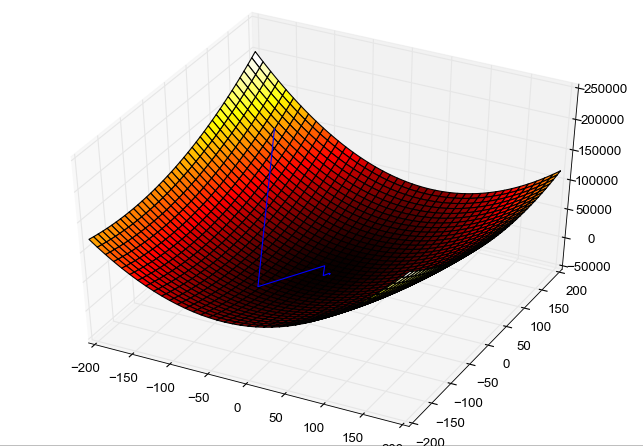
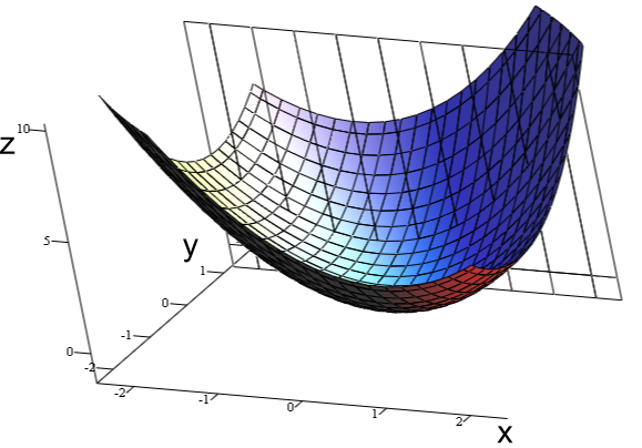
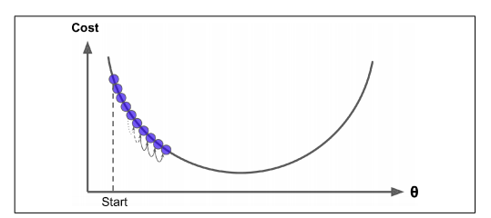
The cost function is a measure of how good our model is at making predictions. The shape of a cost function defines our goal of optimization.
If the shape of the cost function is a convex function, our goal is to find the only minimum. This is relatively simpler cause there is no local minimum and we just need to converge to the global minimum.
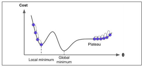
If the shape of the cost function is not a convex function, our goal is to find the lowest possible value in the neighborhood.

Gradient Descent

Gradient descent is a first-order iterative optimization algorithm used to minimize a function L, commonly used in machine learning and deep learning.
It’s a first-order optimization algorithm because, in every iteration, the algorithm takes the first-order derivative for updating the parameters. Parameters refer to coefficients in a regression problem or the weights of a neural network. These parameters are updated by the gradient which gives the direction of the steepest ascent. In every iteration, this is performed by updating parameters in the opposite direction of the gradient computed for cost function L, w.r.t the parameters θ. The size of the update is determined by the step size called learning rate α.
To understand this algorithm, let us consider the case of a person trying to get to the bottom of the valley as quickly as possible.
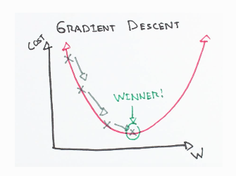
It is obvious that we take the direction of the steepest slope to move down quickly. Now, the question is how do we find this direction? Gradient Descent finds the same by measuring the local gradient of the error function and goes in the opposite direction of the gradient until we reach the global minimum.

As mentioned earlier, the algorithm calculates the gradient of the cost function w.r.t every parameter θ, which tells us the slope of our cost function at our current position (current parameter values) and the direction we should move to update our parameters. The size of our update is controlled by the learning rate.
The most commonly used learning rates are : 0.3, 0.1, 0.03, 0.01, 0.003, 0.001.

Learning Rate α

A high learning rate results in large step sizes. Though there is a chance to reach the bottom-most point quickly, we risk overshooting the global minimum as the slope of the hill is constantly changing.

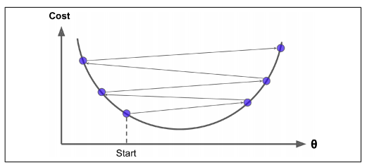
A low learning rate results in small step sizes. Thus, we move in the opposite direction of the gradient precisely. The drawback here is the time required for calculating the gradient. So it will take us a very long time to converge (to reach the bottom-most point).

As mentioned before, our goal is to reach a global minimum. But at times when our cost function has an irregular curve (mostly in the case of deep learning neural networks), with random initialization in place, one might reach a local minimum, which is not as good as the global minimum. One way to overcome this is by using the concept of momentum.

The learning rate affects how quickly our model can converge. Thus the right value means lesser time for us to train the model. This is crucial because lesser training time means lesser GPU run-time.

Normalization

Before performing Gradient Descent, it is important to scale all our feature variables. Feature scaling plays a huge role in the shape of the cost function defined. The Gradient Descent algorithm converges quickly when normalization is performed or contours of cost function would be narrower and taller, which means it would take a longer time to converge.
Normalizing data means scaling the data to attain (mean) μ=0 with (standard deviation) σ=1.
Consider n feature variables. An instance xᵢ can be scaled as follows:

One could use Scikit-Learn’s StandardScaler class to perform feature scaling.

The optimization procedure

Before getting into further details let us define partial derivatives.
In Gradient Descent we compute the gradient of the cost function w.r.t every parameter. This means that we calculate how much the cost function varies when either of the parameters changes. This is called a partial derivative.
Consider a cost function L, with parameters θ. It can be denoted as L(θ). Our goal is to minimize this cost function by finding the best parameter θ values.

We initialize our parameters θ with random values.
We choose a learning rate α and perform feature scaling (normalization).
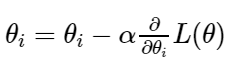
Upon every iteration of the algorithm, we calculate the gradient of cost function w.r.t every parameter and update them as follows:

The negative sign in the optimization step shows that we update our parameters in the opposite direction of the gradient computed for cost function L, w.r.t the parameters θ.
If the gradient is less than 0, we increase the parameters by the value of the gradient multiplied by learning rate α.
If the gradient is greater than 0, we decrease the parameters by the value of the gradient multiplied by learning rate α.
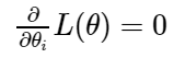
The above steps are repeated until the cost function converges. Now, by the convergence we mean, the gradient of the cost function would be equal to 0.

Types of Gradient Descent

Batch Gradient Descent

Batch Gradient Descent uses a whole batch of training data at every training step. Thus it is very slow for larger datasets.
The learning rate is fixed. In theory, if the cost function has a convex function, it is guaranteed to reach the global minimum, else the local minimum in case the loss function is not convex.

Stochastic Gradient Descent (SGD)

Batch Gradient descent uses a whole batch of the training set in every iteration of training. This is computationally expensive.
Stochastic Gradient Descent (here stochastic means random), takes only a single instance (variance becomes large since we only use 1 example for every iteration of training) randomly and uses the same in every iteration of training. This is really fast but irregular patterns are observed due to the randomness. This randomness is however at times helpful if the cost function is irregular because it can jump out of the local minima with a better chance of finding the global minimum than in Batch Gradient Descent.
We can use a learning rate scheduler set to an initial high value and then gradually decrease our learning rate over time so that we don’t end up bouncing off from a minimum. If the learning rate is reduced too quickly, you may get stuck in a local minimum, or even end up halfway to the minimum. If the learning rate is reduced too slowly, you may jump around the minimum for a long time and end up with a suboptimal solution assuming you halt training too early.
One can use scikit learns SGDRegressor class to implement this.
An important thing to note is we must ensure our training data is shuffled at the beginning of each epoch so the parameters get pulled toward the global optimum, on average. If data is not shuffled, the SGD will not settle close to the global minimum, but instead will optimize label by label.

Mini-batch Gradient Descent

Mini-batch Gradient Descent computes the gradients on small random sets of instances called mini-batches. There is a better chance we can a bit closer to the minimum than Stochastic Gradient Descent but it may be harder for it to escape from local minima.
The batch size can be a power of 2 like 32,64, etc.
Shuffling data like in the case of SGD is recommended to avoid a pre-existing order.
Mini-batch Gradient Descent is faster than Batch Gradient Descent since less number of training examples are used for every training step. It also generalizes better.
The drawback is, it is difficult to converge as one might jump around the minimum region due to the noise present. These oscillations are the reason we need a learning rate decay to decrease the learning rate as move closer to the minimum.

Beyond First Order Optimization

As mentioned earlier, Gradient Descent is a first-order optimization algorithm meaning it only measures the slope of the cost function curve but not the curvature. ( Curvature means the degree by which a curve or a surface deviates from being a straight line or a plane respectively).
So how nature of the function or its curvature measured? It is determined by the second-order derivative. The curvature affects our training.
If the Second-order derivative is equal to 0, the curvature is said to be linear.
If the Second-order derivative is greater than 0, the curvature is said to be moving upward.
If the Second-order derivative is less than 0, the curvature is said to be moving downwards.