8 Linear Regression
"Anyone starting out with Machine Learning algorithms would first come across Linear Regression."
Regression Analysis
-
Before getting into Linear Regression, we must understand what is Regression Analysis.
-
Regression analysis is a set of statistical methods for defining the relationship between a dependent variable and one or more independent variables.
What is Linear Regression?
"Linear Regression is a supervised machine learning algorithm."
- In Linear Regression, we define a relationship between a dependent variable y (output) in terms of one or more independent variables x (inputs) where the representation is a linear equation.
So how is this Linear Regression useful?
-
A linear regression model as mentioned in the beginning is a Supervised Machine Learning algorithm. It is classified as a regression problem. This means that we predict the value of a continuous output variable, which is the dependent variable y (output) with the help of one or more independent variables x (inputs).
-
This is useful to evaluate trends and make predictions or forecasts. Consider the example of a company whose sales have increased every month for the past few years. By building a linear regression model on monthly sales data, one could predict the company’s sales in future months.
- Depending upon the number of independent variables, we have simple and multiple linear regression. Let us look into the same.
Simple Linear Regression
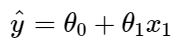
- In Simple Linear Regression, we define the relationship for the dependent variable y (output) for a single independent variable x (input). The representation of the same is a straight line.
Multiple Linear Regression
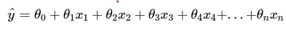
- In Multiple Linear Regression, we define the relationship for the dependent variable y (output) and corresponding two or more independent variables x (inputs).

"So far so good, but what happens when we have non-linearity?"
Polynomial Regression
- In Polynomial Linear Regression, we define the relationship for the dependent variable y (output) and corresponding independent variables x (inputs) as an nth degree polynomial.
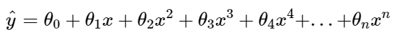
"The Simple and Multiple Linear equations are also Polynomial equations with a single degree, and the Polynomial regression equation is a Linear equation with an nth degree."
-
You may have noticed the unknown parameters (theta). These are the regression coefficients that describe the relationship between the output dependent variable and the independent variables. To simply things, we basically need to find these coefficients and for that, we perform a linear regression to find the best fit line.
-
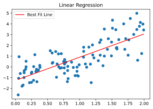
Having discussed the types of linear regression, we can see that “Linear Regression is all about fitting a line” that closely approximates any given point in the dataset. Now, this could be a straight line when the dataset we have is linearly scaled. In the presence of non-linearity, we can make use of Polynomial Regression to fit a curve.
-
Now that you know what is linear regression, let’s start understanding how it is done.
Cost Function
- The cost function tells us how good our model is at making predictions.
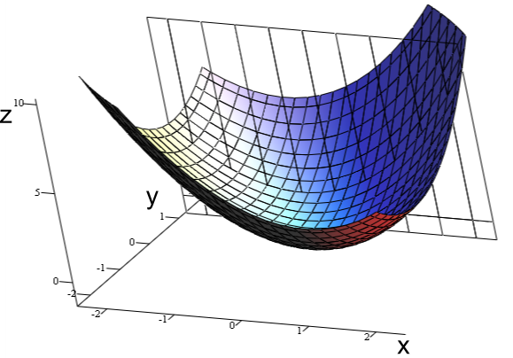
- For the Linear Regression model, we define the cost function MSE (Mean Square Error), which measures the average squared difference between actual and predicted values. Our goal is to minimize this cost function in order to improve the accuracy of the model. It is a convex function, which means that line joining any given 2 points on this never has a local minimum. Only a global minimum.

Training methods of linear regression models
-
There are multiple ways to train a linear regression model.
-
Let us consider a set of data points.
import numpy as np
import matplotlib.pyplot as plt
X = 2 * np.random.rand(100, 1)
y = 2 + 3 * X + np.random.randn(100, 1)
plt.subplot(111)
plt.scatter(X,y)
plt.title('Data Points')
plt.legend(['Random Data'])
plt.show()
- The above code generates a set of random data points. The same can be seen below.
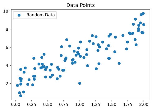
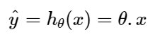
- Now that our data is ready, let us look into methods to fit a regression line. We define the relationship as below.
- Here h is the hypothesis function with n feature represented by vector x.
- Let us look at training methods.
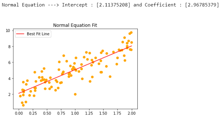
Normal Equation
- The normal equation is regarded as the closed-form. In this method, we can find out the value of unknown parameters θ analytically.
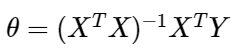
-
In the above equation, θ is the parameter vector that best defines the linear relationship between input feature vector X and target vector Y.
-
Since we invert the matrix of features n, the computational complexity of this method is O(n³).
-
So let us look at the code for the normal equation now.
X_b=np.c_[np.ones((100, 1)),X]
thetas=np.linalg.inv(X_b.T.dot(X_b)).dot(X_b.T).dot(y)
X_new=np.array([[0],[2]])
X_new_b=np.c_[np.ones((2, 1)),X_new]
y_pred_normaleq=X_new_b.dot(thetas)
plt.subplot(111)
plt.scatter(X,y,color='orange')
plt.plot(X_new,y_pred_normaleq,'r-')
plt.title('Normal Equation Fit')
plt.legend(['Best Fit Line'])
print(f"Normal Equation ---> Intercept : {thetas[0]} and Coefficient : {thetas[1]}\n\n")
plt.show()
Pseudoinverse
-
Now, this method is basically used by scikit-learn’s LinearRegression class. This is computed using SVD (Singular Value Decomposition). This is computationally efficient than Normal Equation especially when the matrix X is not invertible (singular).
-
The computational complexity with SVD is O(n²).
-
So let us look at the code for the pseudoinverse now.
from sklearn.linear_model import LinearRegression
regressor=LinearRegression()
regressor.fit(X,y)
y_pred_skl=regressor.predict(X)
plt.subplot(111)
plt.scatter(X,y)
plt.plot(X,y_pred_skl,'r-')
plt.title('Scikit Learn : Linear Regression')
plt.legend(['Best Fit Line'])
print(f"Scikit Learn Linear Regression ---> Intercept : {regressor.intercept_} and Coefficient : {regressor.coef_}\n\n")
plt.show()
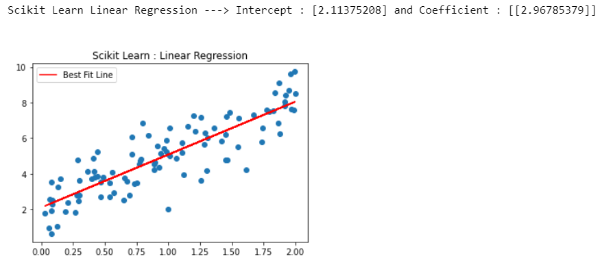
- As you can see, the result is the same for both of the methods.
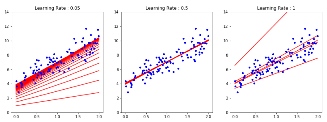
Gradient Descent
-
Gradient descent is a first-order iterative optimization algorithm used to minimize a function L, commonly used in machine learning and deep learning.
-
Am assuming you know the basics of Gradient Descent. However, here is an article on the same. Understanding Gradient Descent
Using Batch Gradient Descent
import numpy as np
import matplotlib.pyplot as plt
X = 2 * np.random.rand(100, 1)
y = 4 + 3 * X + np.random.randn(100, 1)

# Defining a list of tuples of learning rates and subplots
lr = [(0.05,131),(0.5,132),(1,133)]

# number  of iterations
epochs = 100

# Training examples
m = 100

# Parameters
# Considering simple regression
theta = np.random.randn(2,1) # random initialization

# 50 data points
X_b = np.c_[np.ones((100, 1)), X]

# Taking 2 points (extremes) to form our regression line
X_new = np.array([[0], [2]])

# Adding a constant to each since X(0) is 1.
X_new_b = np.c_[np.ones((2, 1)), X_new] # add x0 = 1 to each instance


# The main loop
for lr in lr:
    for iteration in range(epochs):
        gradients = 2/m * X_b.T.dot(X_b.dot(theta) - y)
        theta = theta - lr[0] * gradients
        y_predict = X_new_b.dot(theta)
        plt.figure(1,figsize=(15,5))
        plt.subplot(lr[1])
        plt.plot(X_new, y_predict, "r")
        plt.plot(X, y, "b.")
        plt.ylim((0,14))
        plt.title(f"Learning Rate : {lr[0]}")
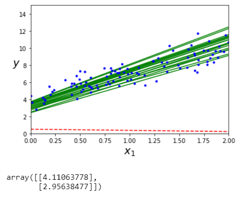
Using Stochastic Gradient Descent
theta_path_sgd = []
m = len(X_b)
np.random.seed(42)
n_epochs = 100
t0, t1 = 5, 50  # learning schedule hyperparameters
def learning_schedule(t):
    return t0 / (t + t1)
theta = np.random.randn(2,1)  # random initialization
for epoch in range(n_epochs):
    for i in range(m):
        if epoch == 0 and i < 20:
            y_predict = X_new_b.dot(theta)
            style = "g-" if i > 0 else "r--"
            plt.plot(X_new, y_predict, style)
        random_index = np.random.randint(m)
        xi = X_b[random_index:random_index+1]
        yi = y[random_index:random_index+1]
        gradients = 2 * xi.T.dot(xi.dot(theta) - yi)
        eta = learning_schedule(epoch * m + i)
        theta = theta - eta * gradients
        theta_path_sgd.append(theta)
plt.plot(X, y, "b.")
plt.xlabel("$x_1$", fontsize=18)
plt.ylabel("$y$", rotation=0, fontsize=18)
plt.axis([0, 2, 0, 15])
plt.show()
Using SGDRegressor class of Scikit Learn
from sklearn.linear_model import SGDRegressor
sgd_reg = SGDRegressor(max_iter=100, tol=1e-3, penalty=None, eta0=0.1, random_state=42)
sgd_reg.fit(X, y.ravel())
sgd_reg.intercept_, sgd_reg.coef_
The output for theta values:
array([4.07441518]), array([2.97048942])