MNIST Handwritten Digits Recognition using PyTorch

![]()
![]()
![]()
![]()
![]()
MNIST dataset
The MNIST database is available at http://yann.lecun.com/exdb/mnist/
The MNIST database is a dataset of handwritten digits. It has 60,000 training samples, and 10,000 test samples. Each image is represented by 28x28 pixels, each containing a value 0 - 255 with its grayscale value.
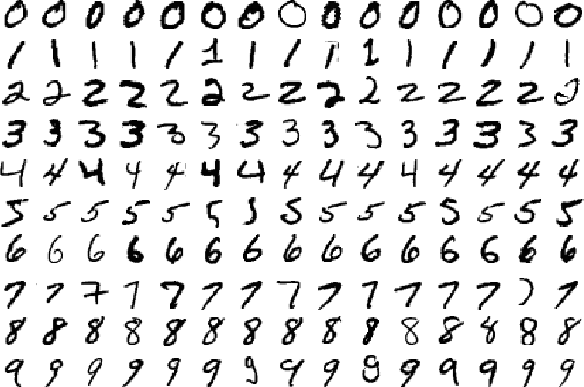
It is a subset of a larger set available from NIST. The digits have been size-normalized and centered in a fixed-size image.
Thanks to Yann LeCun, Corinna Cortes, Christopher J.C. Burges.
Results
A validation dataset of size 12,000 was deduced from the Training dataset with its size being changed to 48,000. We train the following models for 20 epochs.
Prarameters Initialization
- Both models have been initialized with random weights sampled from a normal distribution and bias with 0.
- These parameters have been intialized only for the Linear layers present in both of the models.
- If
nrepresents number of nodes in a Linear Layer, then weights are given as a sample of normal distribution in the range(0,y). Hereyrepresents standard deviation calculated asy=1.0/sqrt(n) - Normal distribution is chosen since the probability of choosing a set of weights closer to zero in the distribution is more than that of the higher values. Unlike in Uniform distribution where probability of choosing any value is equal.
Model - 1 : FFNN
- This
Linear Modeluses 784 nodes at input layer, 512, 256 nodes in the first and second hidden layers respectively, with ouput layer of 10 nodes (10 classes). - The test accuracy is 97.81% (This result uses dropout probability of 20%)
- A
FNet_model.pthfile has been included. With this one can directly load the model state_dict and use for testing.
Model - 2 : CNN
- The
Convolutional Neural Netoworkhas 2 convolution layers and pooling layers with 3 fully connected layers. The first convolution layer takes in a channel of dimension 1 since the images are grayscaled. The kernel size is chosen to be of size 3x3 with stride of 1. The output of this convolution is set to 16 channels which means it will extract 16 feature maps using 16 kernels. We pad the image with a padding size of 1 so that the input and output dimensions are same. The output dimension at this layer will be 16 x 28 x 28. The we apply RelU activation to it followed by a max-pooling layer with kernel size of 2 and stride 2. This down-samples the feature maps to dimension of 16 x 14 x 14. - The second convolution layer will have an input channel size of 16. We choose an output channel size to be 32 which means it will extract 32 feature maps. The kernel size for this layer is 3 with stride 1. We again use a padding size of 1 so that the input and output dimension remain the same. The output dimension at this layer will be 32 x 14 x 14. We then follow up it with a RelU activation and a max-pooling layer with kernel of size 2 and stride 2. This down-samples the feature maps to dimension of 32 x 7 x 7.
- Finally, 3 fully connected layers are used. We will pass a flattened version of the feature maps to the first fully connected layer. The fully connected layers have 1568 nodes at input layer, 512, 256 nodes in the first and second hidden layers respectively, with ouput layer of 10 nodes (10 classes). So we have two fully connected layers of size 1568 x 512 followed up by 512 x 256 and 256 x 10.
- The test accuracy is 99.11% (This result uses dropout probability of 20%)
- A
convNet_model.pthfile has been included. With this one can directly load the model state_dict and use for testing.
MNIST Handwritten Digits Classification
A FFNN (Feed Forward Neural Network) and CNN (Convolutional Nerual Network) have been modeled
Import required packages
import numpy as np
import torch
from torchvision import datasets,transforms
import matplotlib.pyplot as plt
import seaborn as sns
import torch.nn as nn
import torch.nn.functional as F
from torch.utils.data.sampler import SubsetRandomSampler
/usr/local/lib/python3.6/dist-packages/statsmodels/tools/_testing.py:19: FutureWarning: pandas.util.testing is deprecated. Use the functions in the public API at pandas.testing instead.
  import pandas.util.testing as tm
Defining our Transforms
transform=transforms.Compose([transforms.ToTensor()])
Gathering the train and test data
train_data=datasets.MNIST('data',train=True,download=True,transform=transform)
test_data=datasets.MNIST('data',train=False,download=True,transform=transform)
Downloading http://yann.lecun.com/exdb/mnist/train-images-idx3-ubyte.gz to data/MNIST/raw/train-images-idx3-ubyte.gz


HBox(children=(FloatProgress(value=1.0, bar_style='info', max=1.0), HTML(value='')))


Extracting data/MNIST/raw/train-images-idx3-ubyte.gz to data/MNIST/raw
Downloading http://yann.lecun.com/exdb/mnist/train-labels-idx1-ubyte.gz to data/MNIST/raw/train-labels-idx1-ubyte.gz


HBox(children=(FloatProgress(value=1.0, bar_style='info', max=1.0), HTML(value='')))


Extracting data/MNIST/raw/train-labels-idx1-ubyte.gz to data/MNIST/raw
Downloading http://yann.lecun.com/exdb/mnist/t10k-images-idx3-ubyte.gz to data/MNIST/raw/t10k-images-idx3-ubyte.gz


HBox(children=(FloatProgress(value=1.0, bar_style='info', max=1.0), HTML(value='')))


Extracting data/MNIST/raw/t10k-images-idx3-ubyte.gz to data/MNIST/raw
Downloading http://yann.lecun.com/exdb/mnist/t10k-labels-idx1-ubyte.gz to data/MNIST/raw/t10k-labels-idx1-ubyte.gz


HBox(children=(FloatProgress(value=1.0, bar_style='info', max=1.0), HTML(value='')))


Extracting data/MNIST/raw/t10k-labels-idx1-ubyte.gz to data/MNIST/raw
Processing...
Done!


/usr/local/lib/python3.6/dist-packages/torchvision/datasets/mnist.py:469: UserWarning: The given NumPy array is not writeable, and PyTorch does not support non-writeable tensors. This means you can write to the underlying (supposedly non-writeable) NumPy array using the tensor. You may want to copy the array to protect its data or make it writeable before converting it to a tensor. This type of warning will be suppressed for the rest of this program. (Triggered internally at  /pytorch/torch/csrc/utils/tensor_numpy.cpp:141.)
  return torch.from_numpy(parsed.astype(m[2], copy=False)).view(*s)
Defining our Train, Valid and Test Dataloaders
valid_size=0.2

# IMPORTANT
batch_size=20

num_workers=0

train_length = len(train_data)

# obtain training dataset indices that will be used for validation dataset
indices = list(range(train_length))

np.random.shuffle(indices)
split = int(np.floor(valid_size * train_length))
train_idx, valid_idx = indices[split:], indices[:split]

# define samplers for obtaining training and validation batches
train_sampler = SubsetRandomSampler(train_idx)
valid_sampler = SubsetRandomSampler(valid_idx)

# prepare data loaders for train, test and validation dataset
train_loader = torch.utils.data.DataLoader(train_data, batch_size=batch_size,
    sampler=train_sampler, num_workers=num_workers)
valid_loader = torch.utils.data.DataLoader(train_data, batch_size=batch_size,
    sampler=valid_sampler, num_workers=num_workers)
test_loader = torch.utils.data.DataLoader(test_data, batch_size=batch_size,
    num_workers=num_workers)
# This is for debugging
train_idx.__len__(),valid_idx.__len__()
(48000, 12000)
# Printing the length of our train, valid and test dataloaders
# NOTE : Here batch size is 20
len(train_loader),len(valid_loader),len(test_loader)
(2400, 600, 500)
# checking our data
dataiter=iter(train_loader)
images,labels=dataiter.next()
print(images, images.shape, len(images), images[0].shape)
print()
print(labels,labels.shape,len(labels))
tensor([[[[0., 0., 0., ..., 0., 0., 0.],
[0., 0., 0., ..., 0., 0., 0.],
[0., 0., 0., ..., 0., 0., 0.],
...,
[0., 0., 0., ..., 0., 0., 0.],
[0., 0., 0., ..., 0., 0., 0.],
[0., 0., 0., ..., 0., 0., 0.]]],
[[[0., 0., 0., ..., 0., 0., 0.],
[0., 0., 0., ..., 0., 0., 0.],
[0., 0., 0., ..., 0., 0., 0.],
...,
[0., 0., 0., ..., 0., 0., 0.],
[0., 0., 0., ..., 0., 0., 0.],
[0., 0., 0., ..., 0., 0., 0.]]],
[[[0., 0., 0., ..., 0., 0., 0.],
[0., 0., 0., ..., 0., 0., 0.],
[0., 0., 0., ..., 0., 0., 0.],
...,
[0., 0., 0., ..., 0., 0., 0.],
[0., 0., 0., ..., 0., 0., 0.],
[0., 0., 0., ..., 0., 0., 0.]]],
...,
[[[0., 0., 0., ..., 0., 0., 0.],
[0., 0., 0., ..., 0., 0., 0.],
[0., 0., 0., ..., 0., 0., 0.],
...,
[0., 0., 0., ..., 0., 0., 0.],
[0., 0., 0., ..., 0., 0., 0.],
[0., 0., 0., ..., 0., 0., 0.]]],
[[[0., 0., 0., ..., 0., 0., 0.],
[0., 0., 0., ..., 0., 0., 0.],
[0., 0., 0., ..., 0., 0., 0.],
...,
[0., 0., 0., ..., 0., 0., 0.],
[0., 0., 0., ..., 0., 0., 0.],
[0., 0., 0., ..., 0., 0., 0.]]],
[[[0., 0., 0., ..., 0., 0., 0.],
[0., 0., 0., ..., 0., 0., 0.],
[0., 0., 0., ..., 0., 0., 0.],
...,
[0., 0., 0., ..., 0., 0., 0.],
[0., 0., 0., ..., 0., 0., 0.],
[0., 0., 0., ..., 0., 0., 0.]]]]) torch.Size([20, 1, 28, 28]) 20 torch.Size([1, 28, 28])
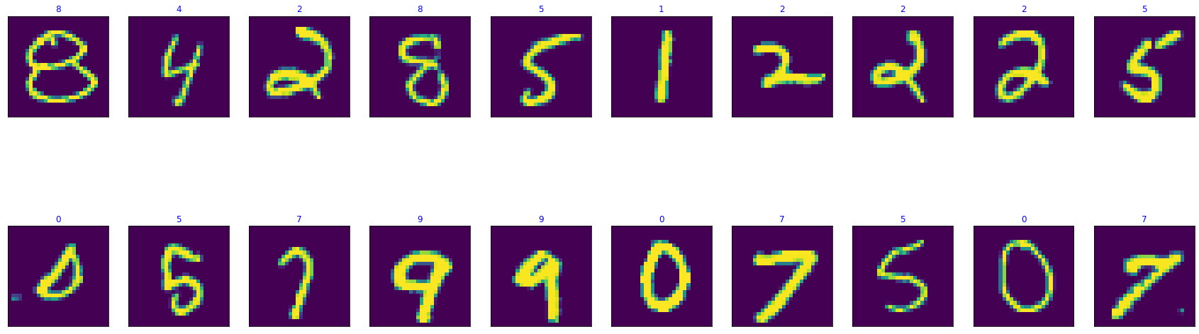
tensor([8, 4, 2, 8, 5, 1, 2, 2, 2, 5, 0, 5, 7, 9, 9, 0, 7, 5, 0, 7]) torch.Size([20]) 20
Visualizing a Training batch
# Displaying images and labels of a batch
fig=plt.figure(figsize=(30,10))
for i in range(len(labels)):
    ax=fig.add_subplot(2,10,i+1,xticks=[],yticks=[])
    plt.imshow(np.squeeze(images[i]))
    ax.set_title(labels[i].item(),color='blue')
Defining our Neural Net Architecture
# Model 1 : This model has dropout set to a certain value
# NOTE : When we want to use dropout we ensure we run train() method on our model --- during training , if not required we should use eval() method --- validation and testing
class FNet(nn.Module):
    def __init__(self):
        super(FNet,self).__init__()
        self.fc1=nn.Linear(784,512)
        self.fc2=nn.Linear(512,256)
        self.out=nn.Linear(256,10)

        # Dropout probability - set for avoiding overfitting
        self.dropout=nn.Dropout(0.2)

    def forward(self,x):
        x = x.view(-1, 28 * 28)
        x=self.dropout(F.relu(self.fc1(x)))
        x=self.dropout(F.relu(self.fc2(x)))
        x=self.out(x)
        return x

class convNet(nn.Module):
  def __init__(self):
    super(convNet,self).__init__()
    self.conv1=nn.Conv2d(in_channels=1,out_channels=16,kernel_size=3,padding=1,stride=1)
    self.conv2=nn.Conv2d(in_channels=16,out_channels=32,kernel_size=3,padding=1,stride=1)
    self.pool=nn.MaxPool2d(kernel_size=2,stride=2)


    self.fc1=nn.Linear(7*7*32,512)
    self.fc2=nn.Linear(512,256)
    self.out=nn.Linear(256,10)
    self.dropout=nn.Dropout(0.2)

  def forward(self,x):
    x=self.pool(F.relu(self.conv1(x)))
    x=self.pool(F.relu(self.conv2(x)))
    x=x.view(-1,7*7*32)
    x = self.dropout(x)
    x=self.dropout(F.relu(self.fc1(x)))
    x=self.dropout(F.relu(self.fc2(x)))
    x=self.out(x)
    return x
model_1=FNet()
model_2=convNet()

def weight_init_normal(m):
    classname=m.__class__.__name__
    if classname.find('Linear')!=-1:
        n = m.in_features
        y = (1.0/np.sqrt(n))
        m.weight.data.normal_(0, y)
        m.bias.data.fill_(0)
model_1.apply(weight_init_normal),model_2.apply(weight_init_normal)
use_cuda=True
if use_cuda and torch.cuda.is_available():
  model_1.cuda()
  model_2.cuda()


print(model_1,'\n\n\n\n',model_2,'\n\n\n\n','On GPU : ',torch.cuda.is_available())
FNet(
  (fc1): Linear(in_features=784, out_features=512, bias=True)
  (fc2): Linear(in_features=512, out_features=256, bias=True)
  (out): Linear(in_features=256, out_features=10, bias=True)
  (dropout): Dropout(p=0.2, inplace=False)
)


 convNet(
  (conv1): Conv2d(1, 16, kernel_size=(3, 3), stride=(1, 1), padding=(1, 1))
  (conv2): Conv2d(16, 32, kernel_size=(3, 3), stride=(1, 1), padding=(1, 1))
  (pool): MaxPool2d(kernel_size=2, stride=2, padding=0, dilation=1, ceil_mode=False)
  (fc1): Linear(in_features=1568, out_features=512, bias=True)
  (fc2): Linear(in_features=512, out_features=256, bias=True)
  (out): Linear(in_features=256, out_features=10, bias=True)
  (dropout): Dropout(p=0.2, inplace=False)
)


 On GPU :  True
Defining our Loss Function
# Loss Function
# If we did not compute softmax at output use nn.CrossentropyLoss() else use nn.NLLLoss()
criterion=nn.CrossEntropyLoss()
Training and Validation Phase
def trainNet(model,lr):
    optimizer=torch.optim.Adam(model.parameters(),lr=lr)


    # Number of epochs to train for
    loss_keeper={'train':[],'valid':[]}
    epochs=20

    # minimum validation loss ----- set initial minimum to infinity
    valid_loss_min = np.Inf

    for epoch in range(epochs):
        train_loss=0.0
        valid_loss=0.0

        """
        TRAINING PHASE
        """
        model.train() # TURN ON DROPOUT for training
        for images,labels in train_loader:
            if use_cuda and torch.cuda.is_available():
                images,labels=images.cuda(),labels.cuda()
            optimizer.zero_grad()
            output=model(images)
            loss=criterion(output,labels)
            loss.backward()
            optimizer.step()
            train_loss+=loss.item()

        """
        VALIDATION PHASE
        """
        model.eval() # TURN OFF DROPOUT for validation
        for images,labels in valid_loader:
            if use_cuda and torch.cuda.is_available():
                images,labels=images.cuda(),labels.cuda()
            output=model(images)
            loss=criterion(output,labels)
            valid_loss+=loss.item()

        # Calculating loss over entire batch size for every epoch
        train_loss = train_loss/len(train_loader)
        valid_loss = valid_loss/len(valid_loader)


        # saving loss values
        loss_keeper['train'].append(train_loss)
        loss_keeper['valid'].append(valid_loss)

        print(f"\nEpoch : {epoch+1}\tTraining Loss : {train_loss}\tValidation Loss : {valid_loss}")
        if valid_loss<=valid_loss_min:
            print(f"Validation loss decreased from : {valid_loss_min} ----> {valid_loss} ----> Saving Model.......")
            z=type(model).__name__
            torch.save(model.state_dict(), z+'_model.pth')
            valid_loss_min=valid_loss
    return(loss_keeper)
m1_loss=trainNet(model_1,0.001)
Epoch : 1	Training Loss : 0.2422629656934684	Validation Loss : 0.13923731955447388
Validation loss decreased from : inf ----> 0.13923731955447388 ----> Saving Model.......

Epoch : 2	Training Loss : 0.12041777377974844	Validation Loss : 0.09333456304622814
Validation loss decreased from : 0.13923731955447388 ----> 0.09333456304622814 ----> Saving Model.......

Epoch : 3	Training Loss : 0.09124215679091321	Validation Loss : 0.08732658982793509
Validation loss decreased from : 0.09333456304622814 ----> 0.08732658982793509 ----> Saving Model.......

Epoch : 4	Training Loss : 0.07515262847801447	Validation Loss : 0.07441183373576375
Validation loss decreased from : 0.08732658982793509 ----> 0.07441183373576375 ----> Saving Model.......

Epoch : 5	Training Loss : 0.06402977682726942	Validation Loss : 0.07680957797386327

Epoch : 6	Training Loss : 0.05664616146977513	Validation Loss : 0.0880538620307046

Epoch : 7	Training Loss : 0.051444328285388016	Validation Loss : 0.08325202515443124

Epoch : 8	Training Loss : 0.04609021995215905	Validation Loss : 0.08688966881602028

Epoch : 9	Training Loss : 0.047100753822042554	Validation Loss : 0.08294352103531423

Epoch : 10	Training Loss : 0.03950506071542602	Validation Loss : 0.09510297800134627

Epoch : 11	Training Loss : 0.041244718991849574	Validation Loss : 0.10204777641329112

Epoch : 12	Training Loss : 0.03726233969181192	Validation Loss : 0.09557511779722253

Epoch : 13	Training Loss : 0.036715185114271846	Validation Loss : 0.10355871919840968

Epoch : 14	Training Loss : 0.03524123047048846	Validation Loss : 0.09944316884041603

Epoch : 15	Training Loss : 0.03153951110024778	Validation Loss : 0.12172619117043518

Epoch : 16	Training Loss : 0.0358803616567481	Validation Loss : 0.12436745904166036

Epoch : 17	Training Loss : 0.032996612528829586	Validation Loss : 0.12394249850443266

Epoch : 18	Training Loss : 0.027076754712408703	Validation Loss : 0.12557926613636103

Epoch : 19	Training Loss : 0.03279251826804246	Validation Loss : 0.13974967400222493

Epoch : 20	Training Loss : 0.03136718728818913	Validation Loss : 0.11489617978800716
m1_loss
{'train': [0.2422629656934684,
  0.12041777377974844,
  0.09124215679091321,
  0.07515262847801447,
  0.06402977682726942,
  0.05664616146977513,
  0.051444328285388016,
  0.04609021995215905,
  0.047100753822042554,
  0.03950506071542602,
  0.041244718991849574,
  0.03726233969181192,
  0.036715185114271846,
  0.03524123047048846,
  0.03153951110024778,
  0.0358803616567481,
  0.032996612528829586,
  0.027076754712408703,
  0.03279251826804246,
  0.03136718728818913],
 'valid': [0.13923731955447388,
  0.09333456304622814,
  0.08732658982793509,
  0.07441183373576375,
  0.07680957797386327,
  0.0880538620307046,
  0.08325202515443124,
  0.08688966881602028,
  0.08294352103531423,
  0.09510297800134627,
  0.10204777641329112,
  0.09557511779722253,
  0.10355871919840968,
  0.09944316884041603,
  0.12172619117043518,
  0.12436745904166036,
  0.12394249850443266,
  0.12557926613636103,
  0.13974967400222493,
  0.11489617978800716]}
m2_loss=trainNet(model_2,0.001)
Epoch : 1	Training Loss : 0.1826872301630768	Validation Loss : 0.06585097063992483
Validation loss decreased from : inf ----> 0.06585097063992483 ----> Saving Model.......

Epoch : 2	Training Loss : 0.0674664011702195	Validation Loss : 0.04612872727685802
Validation loss decreased from : 0.06585097063992483 ----> 0.04612872727685802 ----> Saving Model.......

Epoch : 3	Training Loss : 0.050894734488366185	Validation Loss : 0.03867369514993925
Validation loss decreased from : 0.04612872727685802 ----> 0.03867369514993925 ----> Saving Model.......

Epoch : 4	Training Loss : 0.04129452675137311	Validation Loss : 0.052427549013309545

Epoch : 5	Training Loss : 0.0365402026555545	Validation Loss : 0.04735522323755769

Epoch : 6	Training Loss : 0.03031732397953616	Validation Loss : 0.03929244600439025

Epoch : 7	Training Loss : 0.029407411107780383	Validation Loss : 0.033328903499340944
Validation loss decreased from : 0.03867369514993925 ----> 0.033328903499340944 ----> Saving Model.......

Epoch : 8	Training Loss : 0.02437169043765626	Validation Loss : 0.039428115541503155

Epoch : 9	Training Loss : 0.02453923800847876	Validation Loss : 0.04056901453031609

Epoch : 10	Training Loss : 0.023616162115714334	Validation Loss : 0.05141845186291533

Epoch : 11	Training Loss : 0.021621274729049553	Validation Loss : 0.04135949456253753

Epoch : 12	Training Loss : 0.017968397914148504	Validation Loss : 0.04822746347893704

Epoch : 13	Training Loss : 0.016996163129919167	Validation Loss : 0.04550639333938073

Epoch : 14	Training Loss : 0.017790891666109476	Validation Loss : 0.045940867657337056

Epoch : 15	Training Loss : 0.016738109681809152	Validation Loss : 0.049315622418102154

Epoch : 16	Training Loss : 0.01715114416935609	Validation Loss : 0.04806307668042017

Epoch : 17	Training Loss : 0.016048815001717356	Validation Loss : 0.04278426816728307

Epoch : 18	Training Loss : 0.013644983192738127	Validation Loss : 0.05559660668154593

Epoch : 19	Training Loss : 0.015528520039336536	Validation Loss : 0.06406163931759701

Epoch : 20	Training Loss : 0.013415283101180947	Validation Loss : 0.05390467394411902
m2_loss
{'train': [0.1826872301630768,
  0.0674664011702195,
  0.050894734488366185,
  0.04129452675137311,
  0.0365402026555545,
  0.03031732397953616,
  0.029407411107780383,
  0.02437169043765626,
  0.02453923800847876,
  0.023616162115714334,
  0.021621274729049553,
  0.017968397914148504,
  0.016996163129919167,
  0.017790891666109476,
  0.016738109681809152,
  0.01715114416935609,
  0.016048815001717356,
  0.013644983192738127,
  0.015528520039336536,
  0.013415283101180947],
 'valid': [0.06585097063992483,
  0.04612872727685802,
  0.03867369514993925,
  0.052427549013309545,
  0.04735522323755769,
  0.03929244600439025,
  0.033328903499340944,
  0.039428115541503155,
  0.04056901453031609,
  0.05141845186291533,
  0.04135949456253753,
  0.04822746347893704,
  0.04550639333938073,
  0.045940867657337056,
  0.049315622418102154,
  0.04806307668042017,
  0.04278426816728307,
  0.05559660668154593,
  0.06406163931759701,
  0.05390467394411902]}
Loading model from Lowest Validation Loss
# Loading the model from the lowest validation loss
model_1.load_state_dict(torch.load('FNet_model.pth'))
model_2.load_state_dict(torch.load('convNet_model.pth'))
<All keys matched successfully>
print(model_1.state_dict,'\n\n\n\n',model_2.state_dict)
<bound method Module.state_dict of FNet(
  (fc1): Linear(in_features=784, out_features=512, bias=True)
  (fc2): Linear(in_features=512, out_features=256, bias=True)
  (out): Linear(in_features=256, out_features=10, bias=True)
  (dropout): Dropout(p=0.2, inplace=False)
)>


 <bound method Module.state_dict of convNet(
  (conv1): Conv2d(1, 16, kernel_size=(3, 3), stride=(1, 1), padding=(1, 1))
  (conv2): Conv2d(16, 32, kernel_size=(3, 3), stride=(1, 1), padding=(1, 1))
  (pool): MaxPool2d(kernel_size=2, stride=2, padding=0, dilation=1, ceil_mode=False)
  (fc1): Linear(in_features=1568, out_features=512, bias=True)
  (fc2): Linear(in_features=512, out_features=256, bias=True)
  (out): Linear(in_features=256, out_features=10, bias=True)
  (dropout): Dropout(p=0.2, inplace=False)
)>
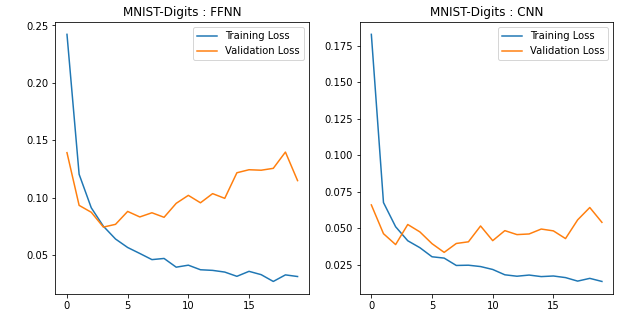
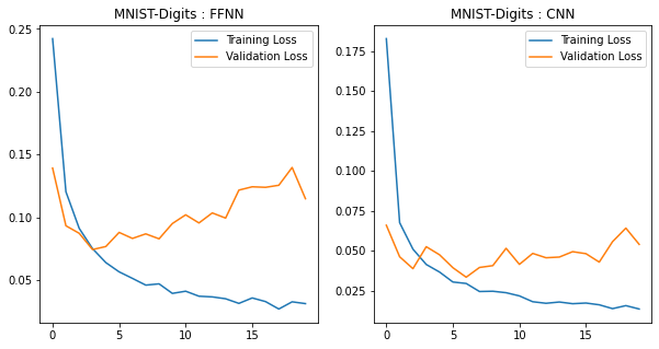
Plotting Training and Validation Losses
title=['FFNN','CNN']
model_losses=[m1_loss,m2_loss]
fig=plt.figure(1,figsize=(10,5))
idx=1
for i in model_losses:
  ax=fig.add_subplot(1,2,idx)
  ax.plot(i['train'],label="Training Loss")
  ax.plot(i['valid'],label="Validation Loss")
  ax.set_title('MNIST-Digits : '+title[idx-1])
  idx+=1
  plt.legend();
Testing Phase
def test(model):
correct=0
test_loss=0
class_correct = list(0. for i in range(10))
class_total = list(0. for i in range(10))
model.eval() # test the model with dropout layers off
for images,labels in test_loader:
if use_cuda and torch.cuda.is_available():
images,labels=images.cuda(),labels.cuda()
output=model(images)
loss=criterion(output,labels)
test_loss+=loss.item()
_,pred=torch.max(output,1)
correct = np.squeeze(pred.eq(labels.data.view_as(pred)))
for i in range(batch_size):
label = labels.data[i]
class_correct[label] += correct[i].item()
class_total[label] += 1
test_loss=test_loss/len(test_loader)
print(f'For {type(model).__name__} :')
print(f"Test Loss: {test_loss}")
print(f"Correctly predicted per class : {class_correct}, Total correctly perdicted : {sum(class_correct)}")
print(f"Total Predictions per class : {class_total}, Total predictions to be made : {sum(class_total)}\n")
for i in range(10):
if class_total[i] > 0:
print(f"Test Accuracy of class {i} : {float(100 * class_correct[i] / class_total[i])}% where {int(np.sum(class_correct[i]))} of {int(np.sum(class_total[i]))} were predicted correctly")
else:
print('Test Accuracy of %5s: N/A (no training examples)' % (classes[i]))
print(f"\nOverall Test Accuracy : {float(100. * np.sum(class_correct) / np.sum(class_total))}% where {int(np.sum(class_correct))} of {int(np.sum(class_total))} were predicted correctly")
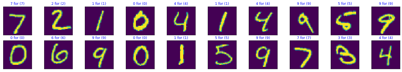
# obtain one batch of test images
dataiter = iter(test_loader)
images, labels = dataiter.next()
# get sample outputs
if use_cuda and torch.cuda.is_available():
images,labels=images.cuda(),labels.cuda()
output = model(images)
# convert output probabilities to predicted class
_, preds = torch.max(output, 1)
# prep images for display
images = images.cpu().numpy()
# plot the images in the batch, along with predicted and true labels
fig = plt.figure(figsize=(25, 4))
for idx in np.arange(20):
ax = fig.add_subplot(2, 20/2, idx+1, xticks=[], yticks=[])
ax.imshow(np.squeeze(images[idx]))
ax.set_title("{} for ({})".format(str(preds[idx].item()), str(labels[idx].item())),
color=("blue" if preds[idx]==labels[idx] else "red"))
Visualizing a Test batch with results
FFNN
test(model_1)
For FNet :
Test Loss: 0.07923624516067411
Correctly predicted per class : [972.0, 1123.0, 1005.0, 987.0, 962.0, 863.0, 929.0, 1009.0, 951.0, 980.0], Total correctly perdicted : 9781.0
Total Predictions per class : [980.0, 1135.0, 1032.0, 1010.0, 982.0, 892.0, 958.0, 1028.0, 974.0, 1009.0], Total predictions to be made : 10000.0

Test Accuracy of class 0 : 99.18367346938776% where 972 of 980 were predicted correctly
Test Accuracy of class 1 : 98.94273127753304% where 1123 of 1135 were predicted correctly
Test Accuracy of class 2 : 97.38372093023256% where 1005 of 1032 were predicted correctly
Test Accuracy of class 3 : 97.72277227722772% where 987 of 1010 were predicted correctly
Test Accuracy of class 4 : 97.9633401221996% where 962 of 982 were predicted correctly
Test Accuracy of class 5 : 96.74887892376681% where 863 of 892 were predicted correctly
Test Accuracy of class 6 : 96.97286012526096% where 929 of 958 were predicted correctly
Test Accuracy of class 7 : 98.15175097276264% where 1009 of 1028 were predicted correctly
Test Accuracy of class 8 : 97.63860369609856% where 951 of 974 were predicted correctly
Test Accuracy of class 9 : 97.12586719524282% where 980 of 1009 were predicted correctly

Overall Test Accuracy : 97.81% where 9781 of 10000 were predicted correctly

CNN
test(model_2)
For convNet :
Test Loss: 0.026931680879527447
Correctly predicted per class : [978.0, 1131.0, 1020.0, 1007.0, 980.0, 879.0, 947.0, 1019.0, 966.0, 984.0], Total correctly perdicted : 9911.0
Total Predictions per class : [980.0, 1135.0, 1032.0, 1010.0, 982.0, 892.0, 958.0, 1028.0, 974.0, 1009.0], Total predictions to be made : 10000.0

Test Accuracy of class 0 : 99.79591836734694% where 978 of 980 were predicted correctly
Test Accuracy of class 1 : 99.64757709251101% where 1131 of 1135 were predicted correctly
Test Accuracy of class 2 : 98.83720930232558% where 1020 of 1032 were predicted correctly
Test Accuracy of class 3 : 99.70297029702971% where 1007 of 1010 were predicted correctly
Test Accuracy of class 4 : 99.79633401221996% where 980 of 982 were predicted correctly
Test Accuracy of class 5 : 98.54260089686099% where 879 of 892 were predicted correctly
Test Accuracy of class 6 : 98.8517745302714% where 947 of 958 were predicted correctly
Test Accuracy of class 7 : 99.12451361867704% where 1019 of 1028 were predicted correctly
Test Accuracy of class 8 : 99.17864476386038% where 966 of 974 were predicted correctly
Test Accuracy of class 9 : 97.52229930624381% where 984 of 1009 were predicted correctly

Overall Test Accuracy : 99.11% where 9911 of 10000 were predicted correctly