7. Learning Curves
"Evaluating machine learning models the right way."
Learning curves are useful in analyzing a machine learning model’s performance over various sample sizes of the training dataset.
Evaluating Models
"Always plot learning curves while evaluating models".
-
Okay, so the basic thing we know is, if a model performs well on the training data but generalizes poorly, then the model is overfitting. If it performs poorly on both, then it is underfitting.
-
The hyperparameters must be set in such a way that, both bias and variance are as low as possible.
How are Learning Curves helpful?
"Learning curves are plots of the model's performance on the training set and the validation set as a function of varying samples of training dataset."
-
To be specific, learning curves show training & validation scores on the y-axis against varying samples of the training dataset on the x-axis.
-
The training & validation scores could be any evaluation metric like MSE, RMSE, etc. on your training and validation sets.
-
Learning curves can be used to understand the bias and variance errors of a model.
Understanding Learning Curves
- Let’s generate some random data, fit a linear regression model for the same, and plot the learning curves for evaluating the model.
from sklearn.linear_model import LinearRegression
from sklearn.model_selection import train_test_split
from sklearn.metrics import mean_squared_error as mse
import numpy as np
import seaborn as sns
import matplotlib.pyplot as plt
plt.style.use('seaborn')
X = 1 * np.random.rand(100, 1)
y = 3 +  3* X + np.random.randn(100, 1)
X_train,X_val,y_train,y_val=train_test_split(X,y,test_size=0.2)
regressor=LinearRegression()
regressor.fit(X_train,y_train)
predictions=regressor.predict(X_val)
plt.figure(1,figsize=(15,5))
plt.subplot(121)
plt.scatter(X,y)
plt.plot(X_val,predictions,color='black')
plt.title('Scikit Learn Linear Regression')
train_errors=[]
val_errors=[]
plt.subplot(122)
for i in range(1,len(X_train)):
    regressor.fit(X_train[:i],y_train[:i])
    train_preds=regressor.predict(X_train[:i])
    val_preds=regressor.predict(X_val)
    train_errors.append(mse(train_preds,y_train[:i]))
    val_errors.append(mse(val_preds,y_val))
plt.plot(range(1,len(X_train)),np.sqrt(train_errors),label='Training error')
plt.plot(range(1,len(X_train)),np.sqrt(val_errors),label='Validation error')
plt.title('Learning Curves')
plt.xlabel('Train set size')
plt.ylabel('RMSE')
plt.legend()
plt.show()
- Look at the output of the above code:
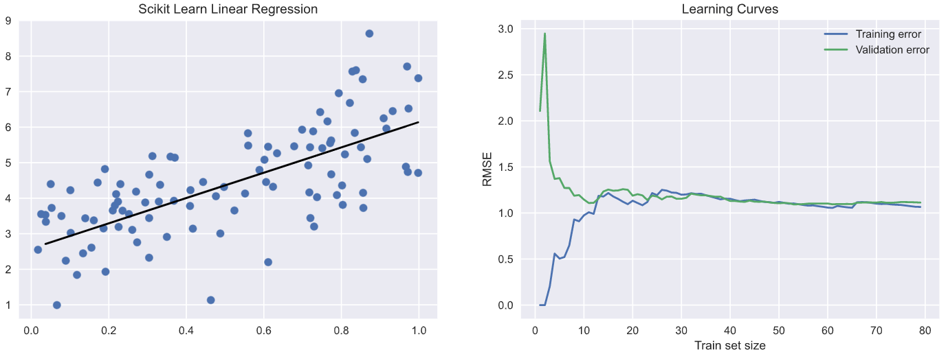
- Okay, nice images. But what is the meaning? It may seem too much at the beginning. Take a look at the following steps to understand the code and the images.
- We generated random data (X,y).
- Derived a training & validation dataset from the same.
- Used Scikit Learn’s LinearRegression class to fit a line for our data, which is what the image on the left is about.
- We then fit the model in the same way as above, but this time, we fit the model for training sample size 1 -> entire training dataset size.
- For every sample size of our training set, we make predictions on our training sample size chosen and the entire validation dataset.
- We calculate the RMSE(Root Mean Square Error) and store the same for plotting later. Done!
-
We can see training & validation scores converge at a particular point. As seen in the image on the right, the first point of convergence w.r.t x-axis is about training sample size 10. This means that, beyond this point, the model will not benefit from increasing the training sample size. Considering the y-axis, the point of convergence is about RMSE value 1. Now, this is okay, and the model seems to generalize properly.
-
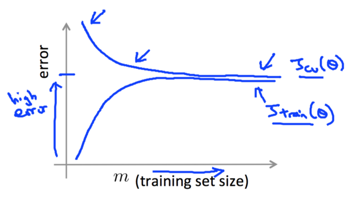
However, take an example where the value at the point of convergence corresponding to the y-axis is high (as seen in the image below). It shows that the model is suffering from high bias. This means that training & validation errors are high and the model doesn’t benefit from increasing the training sample size and thus results in underfitting.
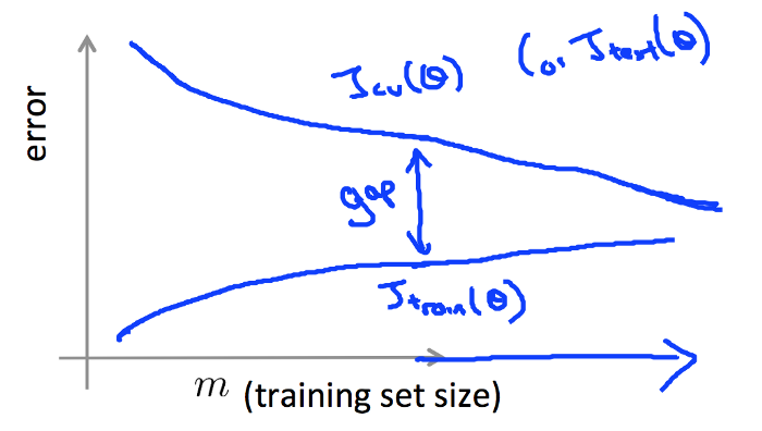
- On the other hand, if there was no visible point of convergence (as seen in the image below), this shows the model is having high variance and has less data. Meaning, the validation errors could be very high and the model would be overfitting.
How to improve model performance?
-
In the case of high bias, increase the number of features, or decrease the regularization parameter, thereby increasing the model complexity.
-
In the case of high variance, decrease the number of features, or increase the regularization parameter, thereby decreasing the model complexity. To fill the gap, just increase the data you have (not the features).